Sparse mode analysis
Analyzing data generated with sparse mode is nearly identical to the dense mode analysis steps, with a few key differences:
The machine learning model file must be provided
The prediction step is performed before calculating synergy
Gather files
Gather the required metadata file and raw file(s), we recommend putting them into separate folders for simplicity:
meta 📂
- Contains the single metadata .csv file
raw 📂
- Contains the raw file(s) in 1536-well format (and nothing else)
Nothing else should be in these folders at the start of analysis.
Deployable ensemble model
Combocat’s ensemble machine learning model is packaged (serialized) and ready to be deployed. As new iterations of models are released, they will be available in the repository’s models folder.
You can read the model file directly into R from the repository:
model_link <- "https://raw.githubusercontent.com/wcwr/combocat/main/models/m03_Feb_2026_02.23PM_Train500_Test167_TuneT.RDS"

my_model <-
readRDS(url(model_link))Check to make sure this is the latest/desired model before loading
Model nomenclature:
The model is a single file and is named according to specific nomenclature which can tell us some useful information. For example, the model m10_Jun_2024_05.00PM_Train552_Test184_TuneT.RDS, can tell us the following:
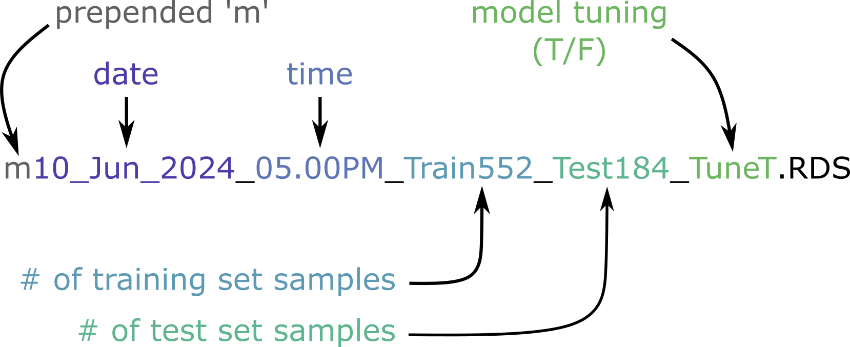
“m” : prepended to all models so files don’t start with numbers
<date>the model was created<time>the model was createdTrain
<number>: Number of samples that were used in the training setTest
<number>: Number of samples that were used in the test setTune
<T/F>: Indicates if hyperparameter tuning of each model was used
The number of training/test set samples also indicates their proportion and the total sample size. 552 + 184 = 736 total samples, indicating a 75/25 split (the default in cc_buildModel)
Quick start
The entire sparse mode analysis can be run in the following single block.
You can try this code yourself by downloading the sparse mode example from GitHub.
#Map, normalize, predict
normData <-
  cc_map(meta_sparse, getwd(), save_raw_plate_heatmaps = TRUE) %>%
  cc_norm(.) %>%
  cc_predict(my_model, .) #Use ensemble model to predict non-measured values

#Fit DR models
drData <-
  cc_getDR(normData)

#Calculate synergy, QC
synData <-
  cc_getSyn(normData, drData) %>%
  cc_getQC(., drData)

#Return/save results
cc_report(
  synData,
  drData,
  cd_plots    = cc_plotMat(synData, "perc_cell_death", color_midpoint = 50),
  syn_plots   = cc_plotMat(synData, "bliss_synergy",   color_midpoint = 20),
extra_plots = cc_plotExtras(synData, color_midpoint = 20))For larger datasets, these steps should be broken up to avoid running out of resources